Foreword
Welcome to the ZK Jargon Decoder 🕵️
The ZK Jargon Decoder aims to be a dictionary and reference guide for common jargon found in cryptography and the zero-knowledge literature. It is collection of informal and practical definitions. Each term should have a one-liner for quick reference and a more detailed explanation if needed.
The nature of this project implies that our definitions will not be perfectly accurate: some technical details will be omitted, some subtleties will be ignored. However if you feel that any of these definitions overlook important aspects of the terms they clarify please get in touch by email or Twitter:
email: nico@zeroknowledge.fm // Twitter: @nico_mnbl
This project is still work in progress, participation and suggestions are always welcome!
License
ZK Jargon Decoder by ZK Jargon Decoder contributors is licensed under CC BY-SA 4.0. To view a copy of this license, visit https://creativecommons.org/licenses/by-sa/4.0/
Introduction to ZK Jargon
Part 1: What does it mean to prove?
This article aims to be a gentle introduction to the notions of decision problems, relations, languages and the complexity class. We follow a running example and rephrase it each time we cover a new term.
Decision Problems
In mathematics, a statement is either TRUE or FALSE.
However, deciding whether a statement is true or false is not always easy.
Consider for example the following statements:
- Statement 1: the number is even.
- Statement 2: the number can be factored.
We can quickly check that Statement 1 is TRUE, but what about Statement 2?
To our knowledge, the best way to decide Statement 2 is just to try factoring .
If we succeed, the statement is TRUE, but we might be trying for a long time, with no guarantee of ever succeeding!
What if we are given additional information? Let’s say we were magically handed (or by luck stumbled upon) the numbers and . We can try to multiply them together and find that indeed . We can now decide Statement 2 ✅.
Notice that with the additional information, we only needed to perform one multiplication; much less work than trying out all the potential factorizations.
In a way, this additional information was in fact a proof that Statement 2 is TRUE.
Answer #1 (informal): proving means giving auxiliary information about a statement to decide that it is true.
We can also rephrase this answer in the form of a condition: a provable statement is one that can be easily decided provided the right information. In complexity theory, this corresponds to the class .
Relations
The discussion above is formalised by the notions of relations and languages:
- A relation is a set of ordered pairs . When talking about relations (provable statements) we refer to the first item, , as an instance, and the second, , as a witness.
Example: factors. Let’s define a relation that we will call . An instance of this relation is an integer, and a witness is an unordered list of integers greater than 1. We will say that the pair is in if and only if contains more than one element and the product of all the elements in is equal to .
For example, the instance has the witness . The instance has multiple witnesses: including , and .
We can now recast Statement 2 in terms of :
- Statement 2 (with jargon, part 1): there exists a witness such that is in .
As we saw above, finding such a witness ourselves is a lot of work. However, given the candidate witness , we can quickly check that the pair is in .
Languages
Rather than always having to say “the instance has a witness such that ”, we use the shorter form “the instance is satisfiable”. Note that the relation which satisfies isn’t explicitly stated and must be made clear from the context.
We can collect all the satisfiable instances of a relation in a set:
- the language defined by a relation is the set of all satisfiable instances for . We often write or .
Example: factors. As we have seen, and are in . On the other hand, prime numbers such as or cannot be expressed as a product of integers. Therefore, they are not in .
Once again we can rephrase Statement 2 in terms of the language defined by :
- Statement 2 (with jargon, part 2): is in .
Answer #2 (same as before, in jargon): proving means giving evidence that an instance is indeed in the language defined by some relation .
More examples. As an exercise, try to cast a Sudoku as a relation and identify the instance, witness and language. What about the relation , defined for some function as all pairs such that ? What happens when we pick to be (i) a polynomial or (ii) a hash function?
Up next: probabilistic and interactive proofs
So far we have only considered the trivial proof system: sending the witness.
In some cases, this is not desirable. Sometimes the witness is private and should remain so. Other times, the witness is just too big to be sent or for the verifier to process. These cases motivate the need for more elaborate (and powerful) proof systems. We discuss these systems more formally in the next article.
Introduction to ZK Jargon
Part 2: Probabilistic and Interactive Proofs
In the previous article, we covered what “proving” means, established some necessary vocabulary and finally discussed the trivial proof system: sending the witness. As discussed, this is not always desirable. Sometimes the witness is private and should remain so. Other times, the witness is just too big to be sent or for the Verifier to process.
In this article, we look at two techniques to build more elaborate proof systems:
- the first is to allow the Verifier to “ask multiple questions”, i.e. to interact with the Prover;
- the second is to allow the Verifier to not read the whole proof.
Naturally, if the proof is shorter than the witness or it is some randomized version of it, the Verifier might sometimes accept proofs for FALSE statements.
This is acceptable (!), as long as it only happens with a small probability.
We call this probability the soundness error (see Soundness).
1. Asking multiple questions
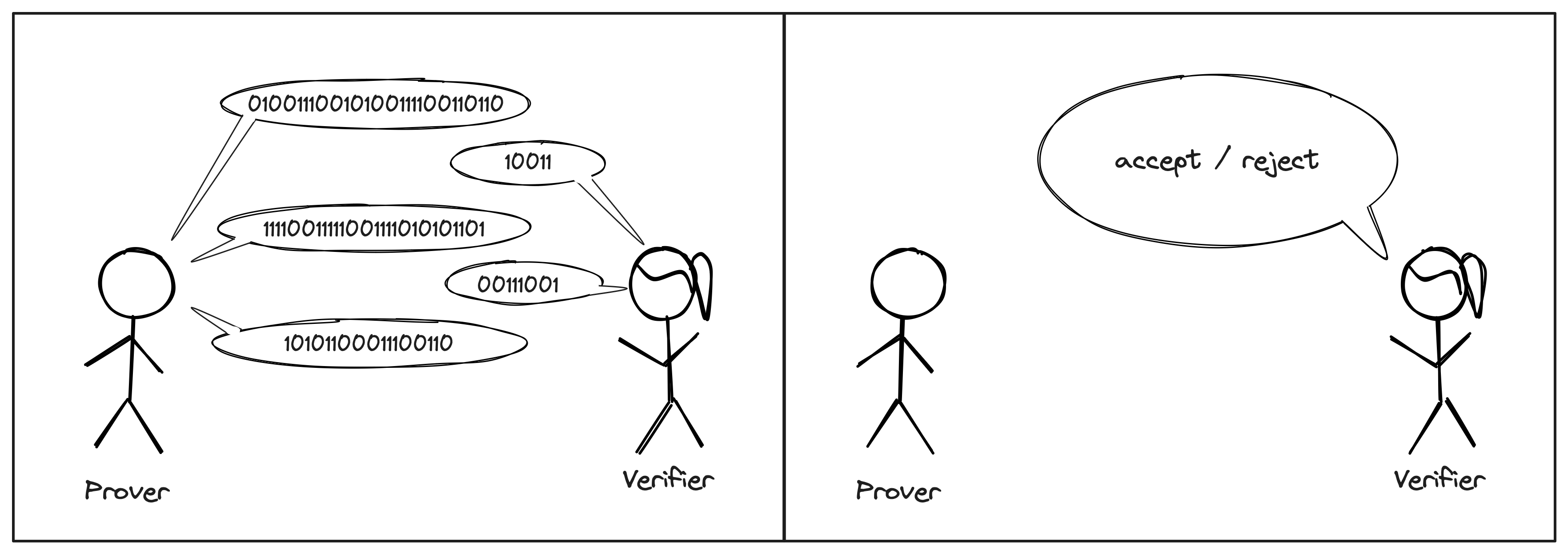
The first technique can be understood as “asking multiple questions”. Rather than sending the witness as a single message, the Prover and Verifier can interact over multiple rounds. This forces the Prover to stay consistent: once something is said, it cannot be unsaid; and any contradiction between the Prover’s messages can be used against him.
Proof systems that use this paradigm are known as interactive proofs (IP).
In practice, we much prefer non-interactive proofs. Luckily, if an IP is such that the Verifier’s messages are all sampled at random from a uniform distribution, there are techniques to transform the IP into a non-interactive proof (e.g., the Fiat-Shamir Transform).
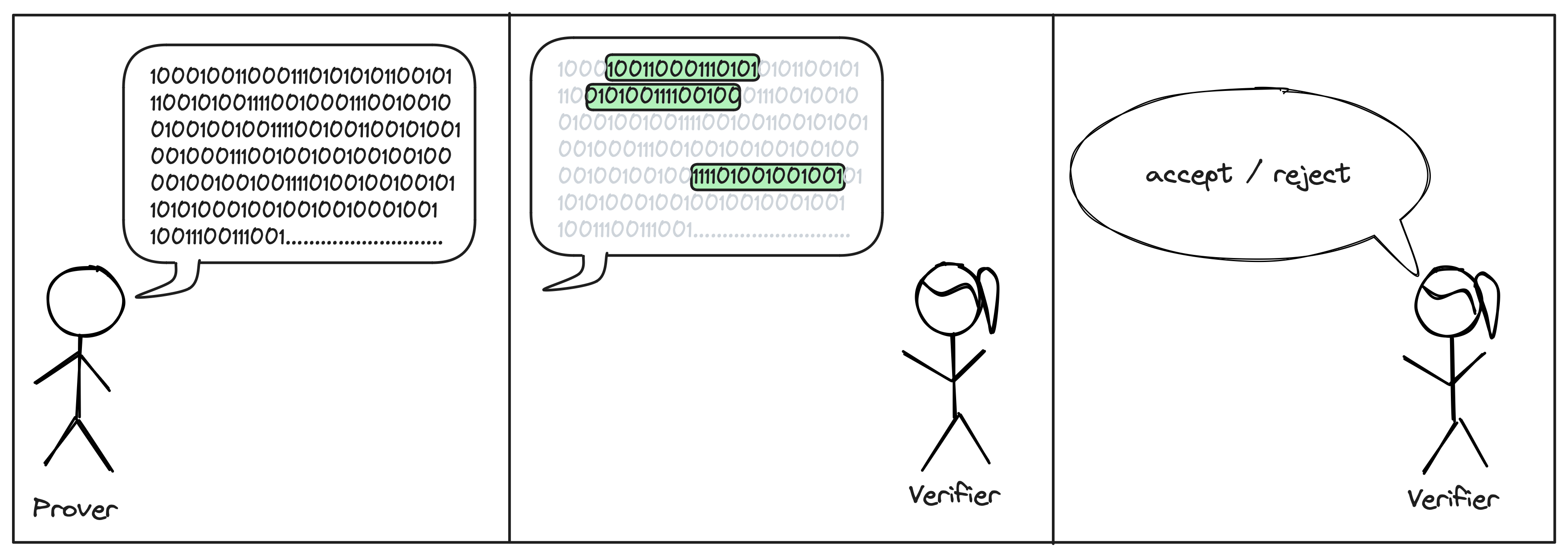
2. Not reading the full proof
The second technique is to not read the full proof. Instead, the Verifier will query the proof at location of her choice. The locations are usually chosen at random after the Prover sent his message.
Proof systems that use this paradigm are known as probabilistically checkable proofs (PCP).
Note that for PCPs to make sense, we need a way for the Prover to send his message, without requiring the Verifier to read it in full. When working on theoretical systems, we allow the Prover to send an oracle for his proof. In this context, an oracle is a black-box that stores the proof string and can be queried at any index. To turn these into real-world systems, we implement the oracle with a commitment scheme.
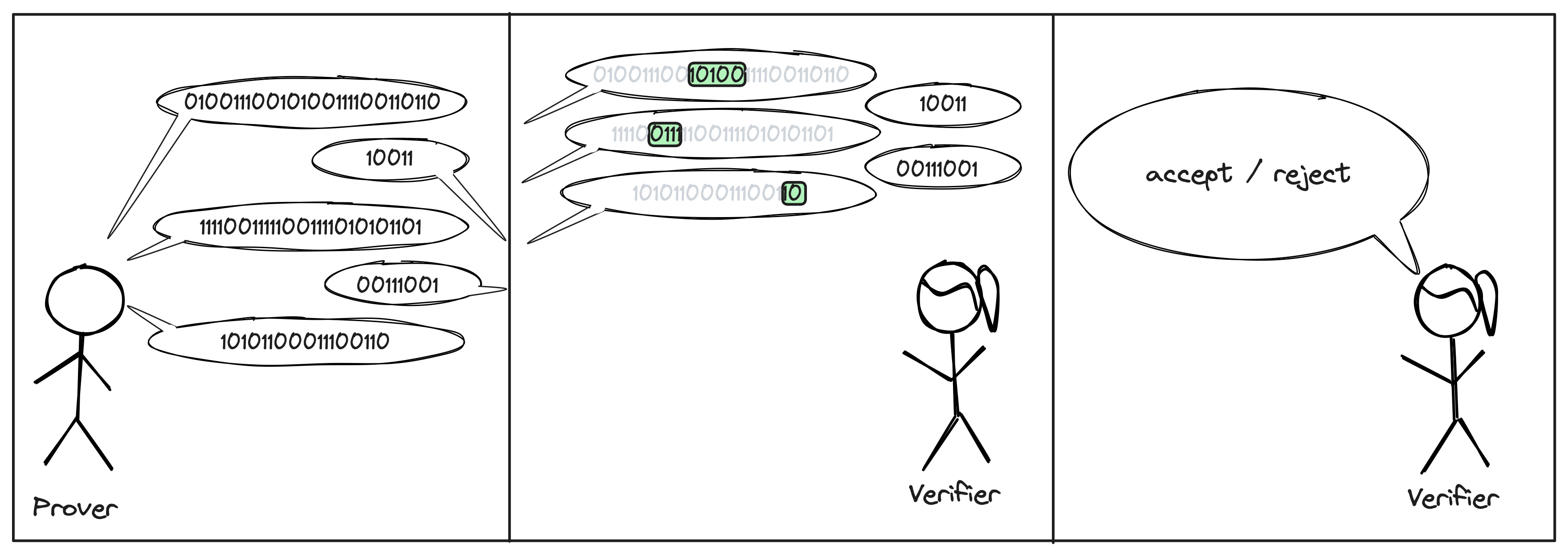
3. Combining both
Of course, we can combine the two above techniques. The resulting proof systems are known as interactive oracle proofs (IOP).
Interestingly, IOPs are not more powerful than PCPs. Everything that can be proven by an IOP can also be proven by a PCP. However, they yield more efficient protocols in practice.
How is this related to my SNARKs?
Our favorite recipe to build a SNARK is as follows: we start with an IOP, replace the theoretical oracles with commitments, and then remove interaction by using the Fiat-Shamir transform. The SNARK “proof” is a collection of commitments to the Prover’s messages, the values of the IOP messages at the locations queried by the Verifier, and some extra information to convince the Verifier that the values do correspond to the committed strings.
For a formal treatment of these techniques, please see the excellent free online book Building Cryptographic Proofs from Hash Functions by Chiesa and Yogev.
References
See ’’Bibliographic Notes“ in Chiesa and Yogev’s Building Cryptographic Proofs from Hash Functions.
Cartoons created in Excalidraw by Nicolas Mohnblatt, using the Stick Figures collection by Youri Tjang and the Speech Bubbles collection by Oscar Capraro.
List of Common Acronyms
Our jargon is full of acronyms. While they are useful to keep communications short and snappy, they can be quite opaque. Especially when they are hard to look up! Below is a list of common acronyms, ordered alphabetically.
A
- AES - advanced encryption standard.
- AGM - algebraic group model.
- AHP - algebraic holographic proof.
- AIR - algebraic intermediate representation.
B
- BARG - batch argument.
- BCS transform- Ben-Sasson–Chiesa–Spooner.
- BLS curves - Barreto–Lynn–Scott.
- BLS signatures - Boneh–Lynn–Sacham.
- BN curves - Barreto–Naehrig.
C
- CCS - customizable constraint system.
- coSNARK - collaborative SNARK.
- CRS - common reference string.
D
- DA - data availability.
- DAS scheme - data availability sampling scheme.
- DEEP - domain extension for the elimination of pretenders.
- DKG - distributed key generation.
- DLOG - discrete logarithm.
- DSA - digital signature algorithm.
- DSL - domain-specific language.
E
- ECC -
- elliptic curve cryptography.
- error-correcting codes.
- ECDSA - elliptic curve digital signature algorithm.
- EdDSA - Edwards-curve digital signature algorithm.
F
- FFT - fast Fourier transform.
- FHE - fully homomorphic encryption.
- FRI - fast Reed-Solomon IOPP of proximity.
- FS transform - Fiat–SHamir transform.
G
- GC - garbled circuit.
- GGM - generic group model.
- GKR protocol - Goldwasser–Kalai–Rothblum.
- GR1CS - generalized rank-1 constraint system.
H
- HE - homomorphic encryption.
- HSM - hardware security module.
I
- iO - indistinguishability obfuscation.
- IOP - interactive oracle proof.
- IOPP - interactive oracle proof of proximity.
- IP - interactive proof.
- IPA - inner-product argument.
- ISA - instruction set architecture.
- IVC - incrementally verifiable computation.
- IZK - interactive zero-knowledge (proof).
J
- JWT - JSON Web Token.
K
- KDF - key-derivation function.
- KEM - key encapsulation mechanism
- KZG commitment - Kate–Zaverucha–Goldberg polynomial commitment scheme.
L
- LPC - list polynomial commitment (scheme).
- LWE - learning with error.
M
- M31 - the Mersenne prime .
- MLE - multilinear extension.
- MNT curves - Miyaji–Nakabayashi–Takano.
- MPC - multi-party computation.
- MPC-TLS - “multi-party computation TLS”, refers to systems that use MPC to attest to the contents of a TLS session.
- MSIS - module short integer solution.
N
- NARG - non-interactive argument.
- NARK - non-interactive argument of knowledge.
- NIZK - non-interactive zero-knowledge proof.
- NTT - number-theoretic transform.
O
- oPRF - oblivious pseudo-random function.
P
- PAIR - pre-processed AIR.
- PCD - proof-carrying data.
- PCP - probabilistically checkable proof.
- PCS - polynomial commitment scheme.
- PESAT relation- polynomial equation satisfaction relation .
- PIOP - polynomial interactive oracle proof.
- PPOT - perpetual powers of tau (trusted setup ceremony).
- PQC - post-quantum cryptography.
- PRF - pseudo-random function.
- PRG - pseudo-random generator.
- PVSS - publicly verifiable secret sharing.
Q
- QAP - quadratic arithmetic program.
- QROM - quantum random oracle model.
R
- R1CS - rank-1 constraint system.
- RAP - randomized AIR with pre-processing (equivalent to PLONKish arithmetization).
- RBR (knowledge) soundness - round-by-round (knowledge) soundness.
- ROM - random oracle model.
- RS code - Reed-Solomon code.
- RSA - Rivest–Shamir–Adleman.
- RTP - real-time proving.
S
- SHA - secure hash algorithm.
- SIS - short integer solution.
- SNARG - succinct non-interactive argument.
- SNARK - succinct non-interactive argument of knowledge.
- SR (knowledge) soundness - state restoration (knowledge) soundness.
- SRS - structured reference string.
- SS - secret sharing.
- SSS - Shamir secret sharing.
- STARK -
- scalable transparent argument of knowledge.
- (colloquial) any proof system that is based on hash functions and error-correcting codes.
T
- TEE - trusted execution environment.
- TFHE - torus fully homomorphic encryption (not to be confused with threshold FHE).
- TLS - transport layer security.
U
- UC - universal composability.
V
- VDF - verifiable delay function.
- VSS - verifiable secret sharing.
W
- WE - witness encryption.
X
- X3DH - extended triple Diffie Hellman (key agreement protocol).
Y
Z
- ZK -
- zero-knowledge.
- (colloquial) any cryptographic proof.
- zkAI - ZK (in the broad “any kind of cryptographic proof” sense) artificial intelligence.
- zkEVM - zero-knowledge Ethereum virtual machine.
- zkID - zero-knowledge identity.
- zkML - ZK (in the broad “any kind of cryptographic proof” sense) machine learning.
- ZKP - ZK proof, both interpretation of the “ZK” acronym are possible.
- zkTLS - “zero-knowledge TLS”, refers to systems that attest to the contents of a TLS session.
- zkVM - zero-knowledge virtual machine.
- zkzk - refers to systems that are zero-knowledge in contexts where “ZK” has been extended to mean “any kind of cryptographic proof”.
0-9
- 2-PC - two-party computation.
Algebraic Holographic Proof (AHP)
An algebraic holographic proof is a interactive proof where the prover sends oracles which are low degree polynomials and can be split into two categories: those that can be processed before the prover-verifier interactions and those that cannot. Closely related to polynomial IOP.
Algebraic Holographic Proofs are first defined in the Marlin paper [CHMMVW20] as a means to separate the information theoretic aspects of SNARKs from the cryptographic aspects. It is an interactive oracle proof with extra properties:
- algebraic: an honest prover only produces oracles for low degree polynomials (just like in polynomial IOPs)
- holographic: the verifier does not need to see the proof’s input (e.g. a circuit) but instead has oracle access to an encoding of it.
We use AHPs, polynomial commitment schemes and the Fiat-Shamir heuristic to construct pre-processing SNARKs such as Marlin and PLONK.
AHP or Polynomial IOP? Algrebraic holographic proofs and polynomial interactive oracle proofs are almost equivalent notions. They were developed concurrently in 2019 by separate research groups: the former by the group behind Marlin [CHMMVW20] and the latter by the group behind DARK [BFS20]. While they formalise very similar proof systems, polynomial IOPs are more general in that they do not require holography (as defined above).
References
[BFS20] Bünz, Benedikt, Ben Fisch, and Alan Szepieniec. “Transparent SNARKs from DARK compilers.” In Advances in Cryptology–EUROCRYPT 2020: 39th Annual International Conference on the Theory and Applications of Cryptographic Techniques, Zagreb, Croatia, May 10–14, 2020, Proceedings, Part I 39, pp. 677-706. Springer International Publishing, 2020.
[CHMMVW20] Chiesa, Alessandro, Yuncong Hu, Mary Maller, Pratyush Mishra, Noah Vesely, and Nicholas Ward. “Marlin: Preprocessing zkSNARKs with universal and updatable SRS.” In Advances in Cryptology–EUROCRYPT 2020: 39th Annual International Conference on the Theory and Applications of Cryptographic Techniques, Zagreb, Croatia, May 10–14, 2020, Proceedings, Part I 39, pp. 738-768. Springer International Publishing, 2020.
Arithmetization
Ambiguous. The process of turning a generic statement or question into a set of equations to be verified or solved - also refers to the output of that process.
Arithmetization is the process of turning a generic statement or question into a set of equation to be verified or solved. Consider the following statement: “I am twice older than my youngest sibling”. Can we write this mathematically? Let’s write the ages of the siblings and the age of the claimant. We can now rewrite the statement as:
To verify the original statement for Alice (8) and her siblings Bob (9) and Charlie (4), we can just plug in the values to our equation. We evaluate each side and determine whether the equation holds: if it holds the statement was true, if it does not the statement was false. Simple as that!
A “good” arithmetization is one in which the final mathematical expressions can be evaluated with minimal effort (computation). While our example was trivial, the process of arithmetization becomes more complex for abstract statements such as: “I have correctly shuffled a deck of cards” or “I know a secret value such that running a public program with as input will output the public value ”.
See also: R1CS, PLONK Arithmetization
Base Field
Elliptic Curve Cryptography. The finite field from which coordinates of an elliptic curve point are chosen.
⚠️ Prerequisites: Finite fields.
See Elliptic Curve.
Circuit
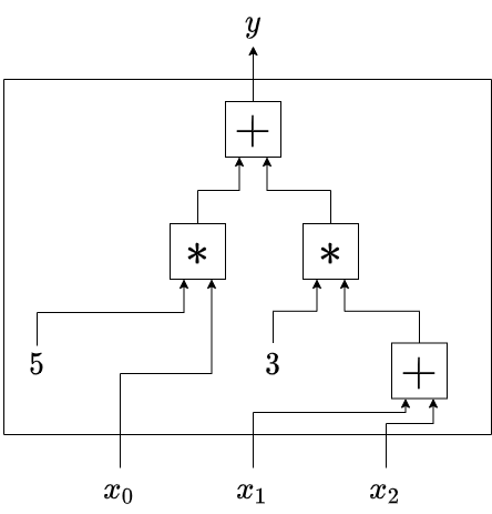
In ZK literature this usually refers to an arithmetic circuit: an ordered collection of additions and multiplications (and sometimes custom operations) that are applied to a set of inputs to yield an output.
The word “circuit” is used somewhat ambiguously, but most of the times we refer to an arithmetic circuit. An arithmetic circuit is an ordered collection of operations (e.g. addition, multiplication) represented by gates. These gates are connected by wires. Given an arithmetic circuit, we can apply an input signal, allow it to propagate through the wires and gates and observe the output. Below is an example of an arithmetic circuit that expects 3 inputs , and , and computes:
Why are we so obsessed with arithmetic circuits? Finding a set of input values that produce a desired output is a hard problem. This problem is known as the circuit satisfiability problem and has been heavily studied in complexity theory. One notable result is that any provable statement can be converted to the satisfiability problem (more formally, the circuit satisfiability problem is NP-complete). This comes in handy when we want to construct proof systems for generic statements.
Coefficient Form
Of a polynomial. Represent a polynomial as a list of the coefficients associated to each power of the indeterminate variable.
Let’s look at an example polynomial , defined as . How can we describe this polynomial in a computer program?
One approach is to record a list of the coefficients in front of every power of the indeterminate : p_coeffs = [5, 0, 4, 1]. Here we ordered the coefficients from lowest to highest power; conveniently, the index of the elements of our array correspond to the power of . As we recorded coefficients, this is known as the “coefficient form”.
Another equivalent representation would be to provide evaluations of at a large enough number of known points (see Evaluation Form).
Coefficient Form vs Evaluation Form.
There is no strictly superior representation. The coefficient form allows for a more lightweight representation of sparse polynomials (polynomials where many of the coefficients are ). Indeed, we only need to record the non-zero coefficients. On the other hand, some operations such as polynomial multiplication are much more expensive in coefficient form () than they are in evaluation form ().
We can convert from coefficient form to evaluation form by evaluating the polynomial at points. The operation that converts from evaluation form back to coefficient form is known as polynomial interpolation (Lagrange interpolation is one way to perform this operation).
Common Reference String
The collection of all public parameters required to run a protocol - usually in the context of SNARKs and polynomial commitment schemes.
In polynomial commitment schemes and SNARKs - like many other cryptographic protocols - different parties need to agree on some common parameters. These often include what kind of mathematical objects they will be manipulating (integers, points on an elliptic curve, lattices, etc…), a prime number, a generator of a cyclic group. Once a setup has been run to determine all the necessary parameters, they are collected into a string and are published for future reference. This collection (string) is what we call a common reference string.
Trusted Setups. In some cases the common parameters are constructed using information that needs to remain secret for the protocol to be secure. In this case we refer to the setup as a Trusted Setup and the string of parameters as a Structured Reference String.
Completeness
Of a proof system. A proof system is complete if, for every
TRUEstatement, the Prover can always produce an accepting proof.
Completeness is a property of a proof system best understood as: “an honest Prover should always be able to convince an honest Verifier of a valid statement”. Here we emphasize that the verifier must be honest. A malicious or faulty verifier (e.g., the implementation has bugs) may reject valid proofs.
Perfect completeness vs Completeness. The definition above imposes that the honest prover always convince the honest verifier (i.e. the probability is 1). We call this property perfect completeness. Sometimes this is not necessary, nor is it achievable. In those cases, we can relax the success probability to be greater than , where is something small.
The math version.
More formally, given a relation and the associated language , the mathematical expression for completeness looks often like the equation below: where and are the honest Prover and Verifier respectively, and denotes the bit output by at the end of the interaction with for the instance .
Constraints
In arithmetized circuits. A constraint is an equation that relates gate inputs to gate outputs.
Elliptic Curve
A set of coordinate pairs that satisfy the equation .
⚠️ Prerequisites: Finite fields.
An elliptic curve is defined as the set of all coordinate pairs such that:
In elliptic curve cryptography, we pick and to be elements of a finite field. We refer to this field as the base field.
We then define a group operation which we call “point addition” and usually denote with the ‘’ symbol. Repeated applications of the group operation can be counted like below:
The number ‘’ above is referred to as a scalar. If we are in a cyclic group, then the scalars also define a finite field: we call this field the scalar field.
Evaluation Form
Of a polynomial. Represent a polynomial as a list of evaluations of the polynomial at given points.
Let’s look at an example polynomial , defined as . How can we describe this polynomial in a computer program?
One approach is to provide evaluations of at a large enough number of known points. In fact, for a polynomial of degree , we will always need at least points. In our case, we could evaluate at 4 points: , , and . We could record this in an array as p_evals = [5, 10, 29, 68]. This recording of evaluations is aptly named the “evaluation form”.
Another equivalent representation would be to provide a list of the coefficients in front of every power of the indeterminate (see Coefficient Form).
Coefficient Form vs Evaluation Form. There is no strictly superior representation. The coefficient form allows for a more lightweight representation of sparse polynomials (polynomials where many of the coefficients are ). Indeed, we only need to record the non-zero coefficients. On the other hand, some operations such as polynomial multiplication are much more expensive in coefficient form () than they are in evaluation form ().
We can convert from coefficient form to evaluation form by evaluating the polynomial at points. The operation that converts from evaluation form back to coefficient form is known as polynomial interpolation (Lagrange interpolation is one way to perform this operation).
Fast Fourier Transform (FFT)
An algorithm that allows us to efficiently “convert” between two equivalent representations of polynomials: either as a list of coefficients (coefficient form) or as a list of evaluations of the polynomial (evaluation form).
COMING SOON.
Fiat-Shamir Heuristic
Turn a public-coin interactive protocol into a non-interactive protocol (in the random oracle model).
A Cautionary Tale. Implementing the Fiat-Shamir heuristic is often a cause for security-critical bugs as described in this Trail of Bits blog post.
Fully Homomorphic Encryption (FHE)
An encryption scheme is said to be fully homomorphic if it allows to compute additions and multiplications on ciphertexts; decrypting the modified ciphertext reveals the result of applying those additions and multiplications to the original message.
Regular encryption allows one party (the sender) to hide a message such that there is only one party (the receiver) that can unhide it.
Fully homomorphic encryption (FHE) adds the possibility of computing an arbitrary function on the ciphertext before it gets decrypted. The decryption will yield .

This process allows to outsource computation to an untrusted party without revealing the input data. Note however that FHE alone gives no guarantees as to what function was run.
Practicality
FHE is regarded as the holy grail of encryption and for a long time was thought to be impossible. Today we are starting to see practical FHE schemes. Note however that they are orders of magnitude slower than symmetric encryption, and non-FHE public key schemes.
Instance
(Of a general purpose SNARK). The public inputs/outputs of a circuit.
In a general purpose SNARK, we call the instance the collection of public values, whether they are inputs, or desired outputs of some computation.
“Instance” is sometimes used interchangeably with the term “statement” although these terms are not exactly the same1.
The terms instance, witness and statement come from complexity theory and the study of relations. Read more in our introductory article
Lagrange Interpolation
A method to construct the unique polynomial of degree that passes through given points.
⚠️ Prerequisites: Coefficient vs Evaluation Form.
Lagrange interpolation is one way to perform polynomial interpolation (recall that this is the process of recovering a polynomial from a set of known evaluations, see prerequisites above).
Let’s say we’ve been given the following point-evaluation pairs , , and . Since we have 4 pairs, we will be able to interpolate the unique polynomial of degree 3 such that for all .
The strategy is the following: for each , we create a polynomial which evaluates to 0 at all the points we were given except , where it evaluates to 1. We can then express the polynomial as:
The set of all polynomials is known as the Lagrange basis for the evaluation domain (here, the set of all values).
Language
See the introductory article on What does it mean to prove?.
Multi-party Computation (MPC)
A protocol that allows mutually distrusting parties, each holding a secret, to jointly compute a function over their secrets without revealing any information other than the result.
As indicated in the name, MPC is a protocol between multiple parties. These parties each hold some data that they want to keep secret. They also do no trust each other but, for some reason, want to jointly compute a program together.
An MPC protocol allows these parties to evaluate the function of interest on their joint private inputs without revealing anything other than the result.
The canonical example: Yao’s millionaire problem.
The example we usually use to illustrate this setting is known as Yao’s millionaire problem, named after its inventor Andrew Yao. Alice and Bob are two millionaires and want to know who is more rich. However they don’t want to reveal how much they own to each other, nor to any third party.The problem can then be extended to allow for more than 2 parties, and any arbitrary program rather than just a comparison of integers.
Generic vs Task-specific Protocols
MPC protocols can be divided into two groups: those that are task-specific, and those that are generic. A generic protocol will allow the set of parties to compute any program they like. However, making the protocol generic prevents it from being optimized for the specific task at hand. On the other hand, task-specific protocols can take advantage fo this specialization and can be overall faster or cheaper to run.
Constructing MPC
Generic 2-party MPC (2-PC) protocols can be built following the garbled circuit approach laid out by Andrew Yao [Yao86]. For further reading on garbled circuits, we recommend A Gentle Introduction to Yao’s Garbled Circuits by Sophia Yakoubov.
Protocols involving more parties will often use techniques such as zero-knowledge proof and fully homomorphic encryption.
Nullifier
A private value which, once revealed, invalidates (or “nullifies”) some associated object.
The term “nullifier” is somewhat loosely defined and appears more in system specs than in academic papers. In general it refers to a private value which, once revealed, invalidates some associated object.
Example: Nullifiers to Prevent Double-Spending
A notorious example system that uses nullifiers is Tornado Cash:
- Users deposit funds into the smart contract and associate a unique, secret nullifier value to their deposit.
- Later one may withdraw from the contract by revealing the nullifier associated with the original deposit. A zero-knowledge proof attests to the fact that the nullifier is associated with one of the contract’s deposits but does not reveal which one.
- Upon successful verification of the nullifier and proof, the smart contract allows the withdrawal.
The smart contract keeps track of all the nullifiers it has seen: if the same nullifier is presented a second time, it must be the case that the funds have already been released and that this user is attempting to cheat by withdrawing more funds than they deposited!
Oracle
Computing. An oracle is a black box that efficiently performs a computation: e.g. a random oracle produces random values, a polynomial oracle evaluates a polynomial at any requested input point.
An oracle is a black box that solves a specific computational problem in constant time. Oracles are used in the theoretical study of computing and complexity theory.
By interacting with an oracle, one can learn the output of the oracle’s computation but learns nothing about its inner workings.
PLONKish Arithmetization
A group of circuit arithmetizations derived from the PLONK paper [GWC19] – their core ingredients are a gate equation and copy constraints that “wire” the gates together.
⚠️ Prerequisites: Arithmetization, Circuit.
PLONK Arithmetization
The PLONK arithmetization was first proposed in the PLONK paper [GWC19] as a means to arithmetize circuits where each gate has 2 inputs and 1 output. Each gate is expressed using a “gate equation”; the wiring is represented as permutations.
(Gate Equation). A single gate with inputs and output is defined by the equation: The values are known as “selectors” and allow us to specialize each gate into enforcing a specific operation. The table below provides some examples:
| Gate Type | Selector Values | Simplified Gate Equation |
|---|---|---|
| Addition | , , , , | |
| Multiplication | , , , , | |
| Public Input is | , , |
(Copy Constraints). Gates are “connected” using copy constraints. Consider two gates for which we want to enforce that the output of the first gate is the left input to the second gate. Let’s label our wires: left input, right input and output of the first gate will be , while left input, right input and output of the second gate will be . To enforce that the value on wire is the same as the value on wire , we show that these values are interchangeable; i.e. that they can be permuted without affecting the validity of the gate equations.
A full PLONK circuit is defined by the matrix of all selector values and the copy permutations.
PLONKish: Variants and Extensions
The PLONK blueprint (gate equation & copy constraints) is extremely versatile and expressive, and has been declined into many variants. The term PLONKish was coined by Daira Hopwood to describe such variants.
Additional features include:
- custom gates - we can add custom functions to the gate equation. To do so we create a new selector and multiply it by some function of the wire values . The new gate equation becomes: .
- larger fan-in and fan-out - the PLONK arithmetization can be extended to support more than 2 inputs and 1 output for each gate.
- lookup tables - the gate equation can also be extended to allow checking that some input value is a member of a table of values.
Some commonly used names for these variants:
- TurboPLONK PLONK arithmetization + custom gates + larger fan-in/fan-out
- PlonkUp [PFMBM22] PLONK arithmetization + lookup tables using plookup.
- UltraPLONK PLONK arithmetization + custom gates + larger fan-in/fan-out + lookup tables using plookup.
- halo2 arithmetization [Zcash] PLONK arithmetization + custom gates + larger fan-in/fan-out + lookup tables using the Halo2 lookup argument.
Additional Resources. In this ZKSummit talk, Zac Williamson, co-author of PLONK, covers the PLONK arithmetization as well as its TurboPLONK extension. The halo2 documentation also provides a thorough explanation of the PLONKish arithmetization used in halo2.
Circuits vs Machine Computation. While the PLONK arithmetization was originally designed to capture arithmetic circuits, its PLONKish extensions are now general enough that they also capture machine computations.
References
[GWC19] Gabizon, Ariel, Zachary J. Williamson, and Oana Ciobotaru. “PLONK: Permutations over Lagrange-bases for Oecumenical Non-interactive arguments of Knowledge.” Cryptology ePrint Archive (2019).
[PFMBM22] Pearson, Luke, Joshua Fitzgerald, Héctor Masip, Marta Bellés-Muñoz, and Jose Luis Muñoz-Tapia. “Plonkup: Reconciling plonk with plookup.” Cryptology ePrint Archive (2022).
[Zcash] Zcash. “The halo2 Book”.
Polynomial Commitment Scheme
A two-phase protocol: in the first phase, a Prover commits to a polynomial by emitting a public commitment; in the second phase the Verifier chooses a value , and the Prover produces a value and convinces the Verifier that .
Overview
A polynomial commitment scheme is a two phase protocol: the first phase is known as the commitment phase, the second as the evaluation phase.
In the commitment phase, a Prover generates a commitment to some polynomial . The type of this commitment object varies depending on the polynomial commitment scheme being used (e.g. a single elliptic curve point for KZG commitments or a vector of elliptic points in IPA commitments).
The evaluation phase is often an interactive protocol between the Prover and a Verifier. The Verifier chooses a point at which it wants to learn the evaluation of . The prover can then produce a value and an “opening proof”. Finally, the Prover and Verifier use the commitment, claimed evaluation and the opening proof as inputs to a (sometimes interactive) protocol to convince the Verifier that .
Properties
We are interested in polynomial commitment schemes that are
- binding: a prover cannot produce false opening proofs for a committed polynomial.
- (optionally) hiding: the commitment reveals nothing about the polynomial.
Some Popular Schemes. KZG (or Kate) commitments, IPA (inner-product argument), FRI (Fast Reed-Solomon Interactive Oracle Proof of Proximity).
Polynomial Interactive Oracle Proof (PIOP)
An interactive proof system in which the prover computes polynomials and the verifier can query these polynomials at evaluation points of her choice.
Polynomial Interactive Oracle Proofs (PIOP, polyIOP or polynomial IOP) emerged from the development of SNARKs and were later formally defined in the DARK paper [BFS20]. These are interactive protocols between a prover and a verifier. With each message the prover produces an oracle and the verifier gets to query any oracles it has received from the prover. In a PIOP, the prover can only produce oracles that evaluate polynomials with degree lower than a given bound.
The following figure is taken from zk-SNARKs: A Gentle Introduction [Nit20]1 and illustrates the prover-verifier interaction in a PIOP:
![PIOP protocol diagram from [Nit20]](definitions/../images/nitulescu-piop.png)
AHP or Polynomial IOP? Algrebraic holographic proofs and polynomial interactive oracle proofs are almost equivalent notions. They were developed concurrently in 2019 by separate research groups: the former by the group behind Marlin [CHMMVW20] and the latter by the group behind DARK [BFS20]. While they formalise very similar proof systems, polynomial IOPs are more general in that they do not require holography (as defined in the AHP article).
References
[BFS20] Bünz, Benedikt, Ben Fisch, and Alan Szepieniec. “Transparent SNARKs from DARK compilers.” In Advances in Cryptology–EUROCRYPT 2020: 39th Annual International Conference on the Theory and Applications of Cryptographic Techniques, Zagreb, Croatia, May 10–14, 2020, Proceedings, Part I 39, pp. 677-706. Springer International Publishing, 2020.
[CHMMVW20] Chiesa, Alessandro, Yuncong Hu, Mary Maller, Pratyush Mishra, Noah Vesely, and Nicholas Ward. “Marlin: Preprocessing zkSNARKs with universal and updatable SRS.” In Advances in Cryptology–EUROCRYPT 2020: 39th Annual International Conference on the Theory and Applications of Cryptographic Techniques, Zagreb, Croatia, May 10–14, 2020, Proceedings, Part I 39, pp. 738-768. Springer International Publishing, 2020.
[Nit20] Anca Nitulescu. zk-SNARKs: a Gentle Introduction. 2020. https://www.di.ens.fr/~nitulesc/files/Survey-SNARKs.pdf.
A great read for the technically-versed and curious reader trying to get a global overview of SNARKs in 2021/2022.
Preprocessing SNARK
A SNARK in which the circuit - or any equivalent description of the computation - is encoded into a proving key and verifying key that are produced ahead of time and independently from any proof.
Public-coin
A public-coin algorithm is an algorithm in which all random values are derived publicly - i.e. without the need for private information or evaluation methods.
Quadratic Arithmetic Program (QAP)
One way (amongst many others) to encode an arithmetic circuit into a set of arithmetic equations. See Arithmetization.
R1CS
Acronym: Rank-1 Constraint System. A circuit arithmetization based on matrix equalities: each matrix row enforces a constraint over linear combinations of the circuit’s wires.
⚠️ Prerequisites: Arithmetization, Circuit.
Rank-1 Constraint Systems (R1CS) are one way (amongst many others) to encode an arithmetic circuit. An R1CS circuit is defined by the following equation: where , and are square matrices of identical sizes, is a vector and ‘’ denotes the element-wise product.
The matrices , and are fixed and define the circuit. To satisfy the R1CS circuit, a prover must find a vector for which the equality above is true. We can also include public inputs by changing the game slightly: we choose a vector of public inputs and require that the prover finds a vector such that the vector satisfies the R1CS equality1. We call the instance vector and the witness vector.
R1CS in Action. You can see R1CS in action in Module 6 of the ZK Whiteboard Sessions from 7:56 to 12:00. There, Mary Maller shows how to populate R1CS matrices to enforce that a value decomposes into three bits by enforcing the following equalities: Note that she is working with a different yet equivalent matrix equation:
Here ‘’ denotes the concatenation operation.
Random Oracle Model (ROM)
An approximation of the real world in which the outputs of certain computations (like hashing or signing a message) are seen as truly random.
The random oracle model is a tool that we use to write security proofs for our cryptographic constructions - it is a representation of the world in which we claim that random oracles exist. A random oracle is a black box to which we ask queries (send values) and receive a response: a value chosen at random. The random oracle’s responses are
- consistent: if I give it a query that it has already seen, the random oracle will give me the same response it gave previously.
- unpredictable: the responses follow a uniform distribution over the oracle’s output domain (this could be integers, strings of 10 characters, points on a curve, etc…).
- unrelated to the query: nothing about a random oracle’s response gives me information about the query.
Hash Functions as Random Oracles. When implementing protocols that are secure in the ROM, we will often claim that cryptographic hash functions (SHA256, Keccak/SHA3, Poseidon) behave like random oracles. This claim usually holds, however we cannot use any hash function. The first ZKHack puzzle explores the dangers of using a poorly-selected hash.
Relation
A relation is a set of pairs ; the condition that makes a pair part of a relation may be arbitrarily defined (“the set of numbers that I think go well together”) or follow some rule (“ is greater than ”).
See the introductory article on What does it mean to prove?.
Roots of Unity
The -th root of unity is a number such that ; we often call roots of unity the set .
The -th root of unity is a number such that . When we use the plural, -th roots of unity, we refer to the set .
Example in the complex numbers
If we were working in a regular (read: not finite) field, the roots of unity would be complex numbers. For example you might already be familiar with the complex number which is in fact the 4-th root of unity in the set of complex numbers (you can check this by computing ). The associated set would be .
Example in a finite field
In a finite field, the definition of “roots of unity” directly maps to that of a multiplicative subgroup of order . For example let’s consider the field with prime characteristic . The elements of this field are , , , , , and . Let’s look at the powers of :
So is the -rd root of unity with the corresponding subgroup of order 3 being .
Scalable
A proof system is scalable if it is succinct and the prover run-time is quasi-linear (i.e. not much longer than running the computation without proving it).
See Succinct.
Scalar Field
Elliptic Curve Cryptography. The finite field defined by counting the number of repeated applications of the group operation (i.e. point addition).
⚠️ Prerequisites: Finite fields.
See Elliptic Curve.
Schwartz-Zippel Lemma
A little mathematical theorem that allows us to assert with high probability whether two polynomials are identical by evaluating both at the same randomly chosen input; this is very efficient!
⚠️ Math: polynomials, probabilities. In the spirit of this “jargon decoder”, we do not look at the lemma directly but instead give informal intuition for why it is useful in ZK arguments
The Schwartz-Zippel lemma is a central component to many arguments of knowledge because it allows us to efficiently check whether two polynomials are identical.
Consider two straight lines (degree 1 polynomials, ): these are either identical or intersect at most once. Similarly, two parabolas (degree 2 polynomials, ) are either identical or will intersect at most twice. Degree 3 polynomials will have at most 3 intersections, etc… The Schwartz-Zippel lemma can be used to show that this pattern is true for polynomials of any degree : their evaluations will only be equal to each other for at most inputs.
With that in mind, imagine that we evaluate two polynomials of degree at most at a single point in some evaluation domain and find that they agree. We know that we are in one of two cases:
- case 1: our polynomials are identical, all their coefficients are the same.
- case 2: our polynomials are different and we are at one of the points where they agree. If our evaluation point was chosen at random in , the probability of finding ourselves in this case is (notation: denotes the order of , i.e. the number of values in the set ). For a sufficiently large compared to , this probability will approach 0.
since case 2 is extremely unlikely we can assert with high probability that the two polynomials were identical.
Formalities - only for those who want them: the lemma itself does not compare polynomials but instead is interested in the probability that a polynomial evaluates to 0. Notice that a non-zero polynomial of degree has at most roots (if it had more roots, it would be of higher degree!). Therefore let be a non-zero polynomial of degree , be the evaluation domain of , and an element of chosen uniformly at random, we can write:
When , this probability is negligible. Therefore if for a value uniformly chosen at random we find that , it is overwhelmingly likely that is the zero polynomial. To check whether two polynomials and are identical, we can check whether the polynomial is the zero polynomial.
SNARK
Acronym: succinct non-interactive argument of knowledge. An argument system in which a Prover can produce a short, single-message proof attesting that she knows some information that shows the truth of a statement.
SNARK is an acronym for Succinct Non-interactive ARgument of Knowledge. The properties are:
- Succinct: the protocol has a proof (and/or verifier) that is smaller than the size of the private inputs and intermediate computation steps. See the article on succinct for further discussion.
- Non-interactive: the protocol only sends one message from the prover to the verifier. The parties don’t even need to be online at the same time!
- Argument of Knowledge: the protocol is an argument and it upholds the knowledge soundness property. At a high level, this means that any computationally bounded prover that produces a valid proof must have known the witness.
Additionally, a SNARK can be publicly verifiable. The prover emits one proof that can then be verified by any third party.
SNARKs are the tool of choice for applications that require creating trust in an asymmetric computation setting. It allows a powerful but untrusted party (the prover) to convince a less powerful party (the verifier) that it performed some computation correctly.
Soundness
Of a proof system. A proof system is sound if, for every
FALSEstatement, the Prover can (almost) never produce an accepting proof.
Soundness is a property of a proof system best understood as: “a malicious Prover should not be able to convince an honest Verifier of an invalid statement”.
The math version.
More formally, given a relation and the associated language , the mathematical expression for soundness looks often like the equation below: where is any malicious prover, is the honest Verifier, denotes the bit output by at the end of the interaction with for the instance and is a small number. We call the soundness error.
Statistical vs Computational Soundness. The notion of soundness described above is known as statistical soundness or information-theoretic soundness. It considers all possible adversaries, including those with unlimited resources. In most real-world applications, we are only concerned with bounded adversaries: we usually limit ourselves to adversaries running probabilistic polynomial-time algorithms. This adversarial model is formalised by the notion of an argument (rather than a “proof”) and that of computational soundness. Computational soundness is defined in the same way as information-theoretic soundness but is only required to hold against probabilistic polynomial-time adversaries.
Stronger Soundness variations
Soundness comes in several levels of strength. Above is the most basic version according to which an honest verifier should only accept a proof if it corresponds to a valid statement. The following describes increasingly stronger versions of soundness.
Knowledge Soundness
When constructing arguments of knowledge, a notion stronger than simple soundness is required: knowledge soundness. In this strengthened scenario, an honest verifier should only accept a proof if it corresponds to a valid statement and it was generated by a prover who knows a valid witness for this statement.
Formally, this is defined in terms of an extractor: an argument system is said to be knowledge sound if there exists an efficient algorithm that, given the prover’s algorithm and internal state, can extract a valid witness for the proven statement. Intuitively, this models the desired property that the prover “knows” a witness for this statement.
Simulation Knowledge Soundness (or Simulation-Extractability)
Another useful and even stronger notion of soundness is simulation-extractability. Informally, it states that an honest verifier should only accept a proof if it corresponds to a valid statement and was generated by a prover who knows a valid witness, even if the prover is allowed to observe honestly generated proofs for arbitrary statements.
Intuitively, if an argument system is simulation-extractable, then it is non-malleable: an adversary can’t observe a proof for some statement generated by a third party and maul it into a proof for another statement for which the adversary does not know a valid witness.
This captures many real-world scenarios where honestly generated proofs are made public and may be seen by potential attackers. As such, it has become the “gold standard” in terms of security notions
STARK
Overloaded. The term STARK has been used to mean:
- the hash-based SNARK of Ben-Sasson et al. [BBHR18],
- any argument of knowledge with a small proof and verifier, a quasi-linear prover and a transparent setup, (could be interactive or non-interactive) or
- any hash-based transparent SNARK.
Origins
“STARK” was first introduced by Ben-Sasson et al. [BBHR18] as an acronym for scalable, transparent argument of knowledge. The properties are:
- Scalable: the protocol is succinct1 and has a quasi-linear prover.
- Transparent: the protocol has a transparent setup; that is, one that does not require secret information.
- Argument of Knowledge: the protocol is an argument and it upholds the knowledge soundness property. At a high level, this means that any computationally bounded prover that produces a valid proof must have known the witness.
Notice that “STARK” says nothing about whether the proof should be non-interactive.
The Ben-Sasson et al. paper [BBHR18] also introduce a concrete protocol that met these properties. By extension, this protocol came to be known as “STARK”.
Evolution
The STARK protocol of Ben-Sasson et al. [BBHR18] was iterated upon and has changed throughout the years. Techniques such as using quotient polynomials, copy constraints and/or lookup tables have made their way into stwo, the latest iteration of StarkWare’s “STARK” proof system. In this manner, today’s “STARK” is essentially a PLONKish protocol with a hash-based polynomial proximity test (e.g., FRI, STIR, WHIR).
Hash-based SNARKs
Today, people use the term “STARK” to mean “any transparent SNARK that relies only on hash functions”. This includes protocols such as Brakedown, Orion and Binius — which by some definitions are not succinct (!).
Disambiguation
Summarizing, we have three possible definitions of “STARK”:
- the hash-based SNARK of Ben-Sasson et al. [BBHR18],
- any argument of knowledge with a small proof and verifier, a quasi-linear prover and a transparent setup, (could be interactive or non-interactive) or
- any hash-based transparent SNARK.
Most of the time it will be up to you to understand from the context what people mean when they say “STARK”. Although it is very rare that people will use STARK to refer to an interactive proof.
Just for fun I’m including a little Venn diagram of what is and isn’t a STARK based on the many definitions.

Naming recommendation. In this book we will use:
- “STARK [BBHR18]” to refer to the transparent SNARK of Ben-Sasson et al.,
- “STARK” to mean “scalable, transparent argument of knowledge”; this could include Nova, Bulletproofs (both transparent SNARKs) and possibly some interactive arguments of knowledge that meet the “scalability” requirement,
- “pure ROM SNARKs”, “hash-based SNARK” or “transparent hash-based SNARK” to mean SNARKs that use hash functions and no other cryptographic primitive; this includes STARK [BBHR18], Ligero, Binius, PLONK+FRI (Redshift, Plonky2).
See the linked article for the variations on that definition.
Structured Reference String
A collection of public parameters for a protocol which were created using information that must remain secret to ensure the protocol’s security.
See Common Reference String and the note at the bottom of the page.
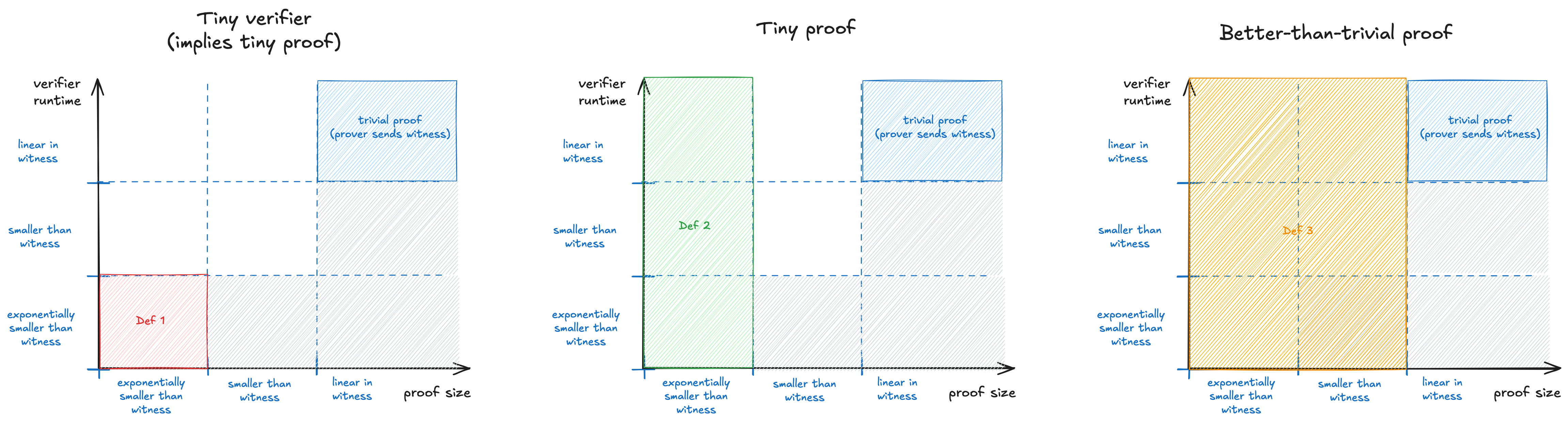
Succinct
Ambiguous. A proof system is succinct if its proof (or verifier) is “smaller” than the size of the private inputs and intermediate computation steps (i.e. the witness); how small changes from one definition to the other.
We say that a proof system is succinct if its proof (or verifier) is “smaller” than the size of the private inputs and intermediate computation steps (i.e. the witness).
However, “small” has been used to mean different things is different contexts. Here are the main options:
- Tiny verifier. The verifier has to be exponentially faster than running the full computation. It also implies that the messages it reads (the proof) are also exponentially smaller than the witness. This definition is the earliest one to appear and also the strictest to satisfy. It is used in textbooks such as the SNARGs Book of Chiesa and Yogev.
- Tiny proof. The proof has to be exponentially smaller than the witness, however we allow the verifier to run in time that is comparable to the full computation.
- Better-than-trivial proof. The proof has to be asymptotically smaller than the witness. The verifier is still allowed to run in time that is comparable to the full computation. This definition is the most relaxed. It is promoted in more recent papers and recommended by Justin Thaler in his 17 misconceptions post.
The image below summarizes these definitions and highlights how they get progressively more relaxed. You can click on the image to expand it.
Examples. Here are some examples of systems that satisfy the definitions:
- Groth16, Plonk+KZG, Plonk+FRI, STARK [BBHR18] all satisfy definitions 1, 2 and 3.
- Bulletproofs, Plonk+IPA / Halo2 satisfy definitions 2 and 3, but do not satisfy definition 1. Their proofs are exponentially smaller, but their verifiers run in linear-time.
- Brakedown, Orion, Binius satisfy definition 3, but not definitions 1 and 2. Their proof size and verifier runtime scale with the square root of the witness.
Threshold Encryption
A public-key encryption scheme in which the secret key is shared amongst parties: to decrypt a ciphertext, we require that a group of strictly more than participants collaborate; is called the threshold.
Transparent Setup
An algorithm that determines a protocol’s public parameters using only public information.
See Common Reference String. Opposite to a trusted setup.
Trusted Setup
An algorithm that determines a protocol’s public parameters using information that must remain secret to ensure the protocol’s security.
See Common Reference String and the note at the bottom of the page. Opposite to a transparent setup.
Vanishing Polynomial
The unique polynomial of degree that evaluates to at all points of a domain of size .
The vanishing polynomial over a set , often denoted , is the polynomial which has a single root at each element of . It can be explicitly written as:
By definition, the vanishing polynomial over will have the following properties:
- it is unique.
- it is of degree .
- for all , . (Hence the name vanishing!)
Vanishing Polynomial for Roots of Unity. When the set is a set of -th roots of unity, the vanishing polynomial can be expressed as: To see why this is the case, let’s consider the set which we know are the -rd roots of unity in (see the Roots of Unity article): Why does this matter? Expressing in this way makes it very efficient to evaluate it at one point!
Witness
(Of a general purpose SNARK). All the circuit variables that the verifier does not see: the prover’s private inputs and all the intermediate values computed in the circuit.
In a general purpose SNARK, we call the witness the collection of values that the verifier does not read; either because they are private to the prover, or because they are too long to satisfy the succinctness property.
Consider the following example:
Peggy sends a string
stringto Victor and wants to convince him that she knows a secret valueseedsuch that applying theKeccakhash 1000 times to it producesstring. That is,string = Keccak(Keccak(...(Keccak(seed)...))).Peggy and Victor therefore agree on a SNARK circuit that takes
seedas a private input andstringas a public input. The circuit applies Keccak once toseedto produce a 1st intermediate value. This value is then fed into Keccak again, producing another intermediate value. This process is repeated 1000 times until a final value is produced. Finally, this last value is compared tostring.
In this example, Peggy wants to keep the value seed secret, so it must certainly be part of the witness. Secondly, notice that the circuit produces 1000 intermediate values. Victor (rightfully so) doesn’t care about these values and shouldn’t have to read through them! He just wants to see string and a short proof that Peggy is saying the truth. So the 1000 intermediate values are also part of the witness.
Witness Encryption
An encryption scheme where public keys are instances (public inputs of a circuits) and private keys are witnesses (the private inputs and intermediate computation steps).
Witness encryption is a generalization of public key encryption.
Recall that for public key encryption, we pick one specific hard problem to generate private-public key pairs. For example, if we choose the discrete logarithm in elliptic curves (EC), the private key is a scalar and the public key is a point . We assume that finding given is hard and use this fact to construct encryption schemes.
In witness encryption, we allow to encrypt to any -problem (see Decision Problems). For example, we could encrypt to an arithmetic circuit — the same ones we use for SNARKs (!). The public key would be the public inputs, while the private key is the private inputs and all intermediate computation steps.
More formally, the public key is any instance of an relation, and the private key is a corresponding witness. Note that depending on the relation, a single public key (instance) could have multiple private keys (witnesses). Depending on your use case this could be a nasty bug or a great feature!
Here is a table summarizing the above discussion:
| Scheme | Hard Problem | Public Key | Private Key |
|---|---|---|---|
| EC public key encryption | EC discrete logarithm | Point | Scalar |
| Circuit-based encryption | Circuit satisfiability | public inputs | private inputs and intermediate wires |
| Generic witness encryption | any -problem | instance | witness |
Witness Encryption in Practice
Witness encryption schemes are not yet practical. Cryptographers are hard at work to make these schemes usable.
However, we do have variants that are already available:
- commitment-based witness encryption (CWE). In CWE, the public key is an instance and a commitment . The corresponding private key is a value such that was a commitment to and was a valid witness for .
CWE example. Following our circuit example: the public key would be the public inputs and a commitment to the private inputs + intermediate steps.
- signature-based witness encryption (SWE). In SWE, the public key is a signature key and a string
s. The corresponding private key is a signature onsby the secret key that corresponds to .SWE example. SWE has been used to build timelock encryption, otherwise known as “encrypting to the future” [DHMW22] [GMR23].
Zero-knowledge Proof
A proof that reveals no more information than the validity of the statement it supports.
A proof is said to be “zero-knowledge” if it does not reveal any information beyond the fact that a statement is TRUE.
Zero-knowledge proofs provide privacy for the prover. Any other proof system is bound to leak at least 1 bit of information, which could have very subtle privacy and security implications.
See S2M1 of the ZK Whiteboard Sessions for an in-depth treatment of how we define zero-knowledge mathematically and prove it.
Warning: implementation bugs. Zero-knowledge is only shown to hold for honest provers. A malicious or faulty prover (e.g., the implementation has bugs) may produce proofs that leak information about the private input.
zkVM
A special type of circuit that implements a CPU; allowing this single circuit to run any program it is given as input.